Originally, I really wanted to do a text mining package related to law but it was becoming too complex and I had like 6 steps and cleaning the data before was a mess. I honestly plan on picking this R package back up in the summer and trying to make it work.

The R package(s) that I did for the final project include a temperature conversion package and a “fun” Chipotle ordering package.

https://github.com/mslement/TempConversion

https://github.com/mslement/Chipotle

Links to my GitHub Repositories to download my packages

Resources I used to create the R packages:

https://hilaryparker.com/2014/04/29/writing-an-r-package-from-scratch/ (provided by Dr.Friedman)

https://www.youtube.com/watch?v=9PyQlbAEujY (video that is literally amazing to follow and was the only thing that made my R package “Build & Reload”

Basically I followed the video linked to create my R projects and packages. The only thing that I had trouble with was with making the DESCRIPTION file but with some research I was able to fix it.

> load_all()

Error: No root directory found in /Users/michelleslement/Desktop/R Programming/Final Project/Chipotle or its parent directories. Root criterion: contains a file `DESCRIPTION`

> use_description() #FIXED

R Code showing my troubles with creating DESCRIPTION file

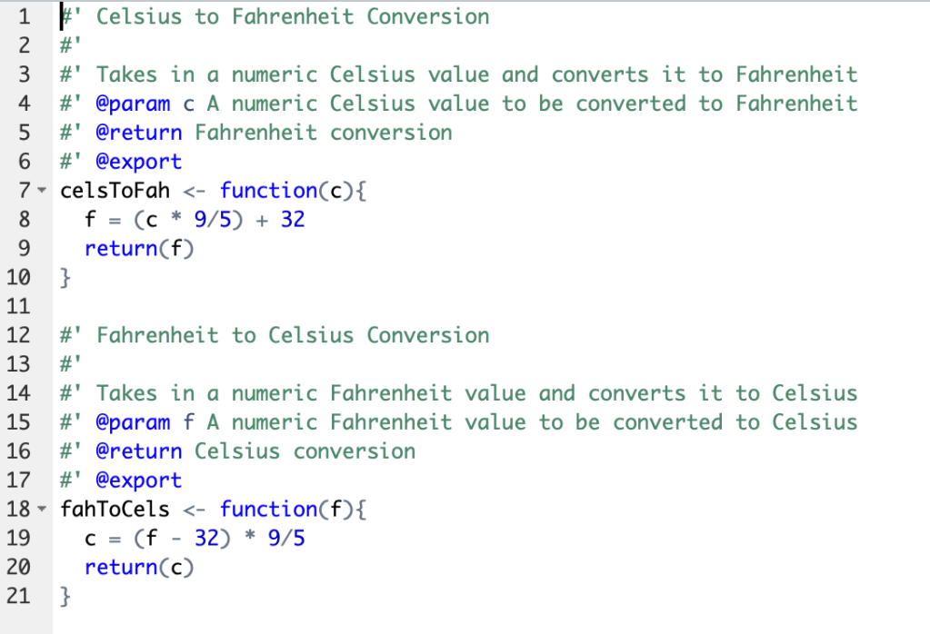
So, my first R package that I made included simple functions to convert Celsius to Fahrenheit(celsToFah(s)) and Fahrenheit to Celsius(fahToCels(f)).

These were very simple functions and I realized that there are literally at least 10 on the internet as examples and I need to think of something unique.

So, that brings me to my second package: Chipotle

This R package that I made included simple functions that displayed the menu(menuDisplay()) and one to order and show the price of the order(orderBowl(meat, rice, bean, top, extraTop)).

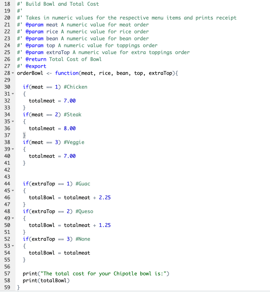
The conversion package is honestly more useful. But after I did my peer reviews, I wanted to do something more fun.

Also, the downfall to the second package is that you can’t implement a data set within the function like you can with the temperature conversion one.

Examples of uses of both packages are in the README files in my GitHub.

GitHub Repository Link(I also uploaded the html): https://github.com/mslement/IntroRProgrammingSlement/blob/master/RMarkdownTest.Rmd

After watching the two videos in the module, I followed the “R Markdown Cheat Sheet” and “R Markdown Reference Guide” provided in the module.

file:///Users/michelleslement/Downloads/rmarkdown-cheatsheet.pdf

file:///Users/michelleslement/Downloads/rmarkdown-reference.pdf

I was not sure if this was supposed to be for our final project or we were supposed to make something up to put in the R Markdown.

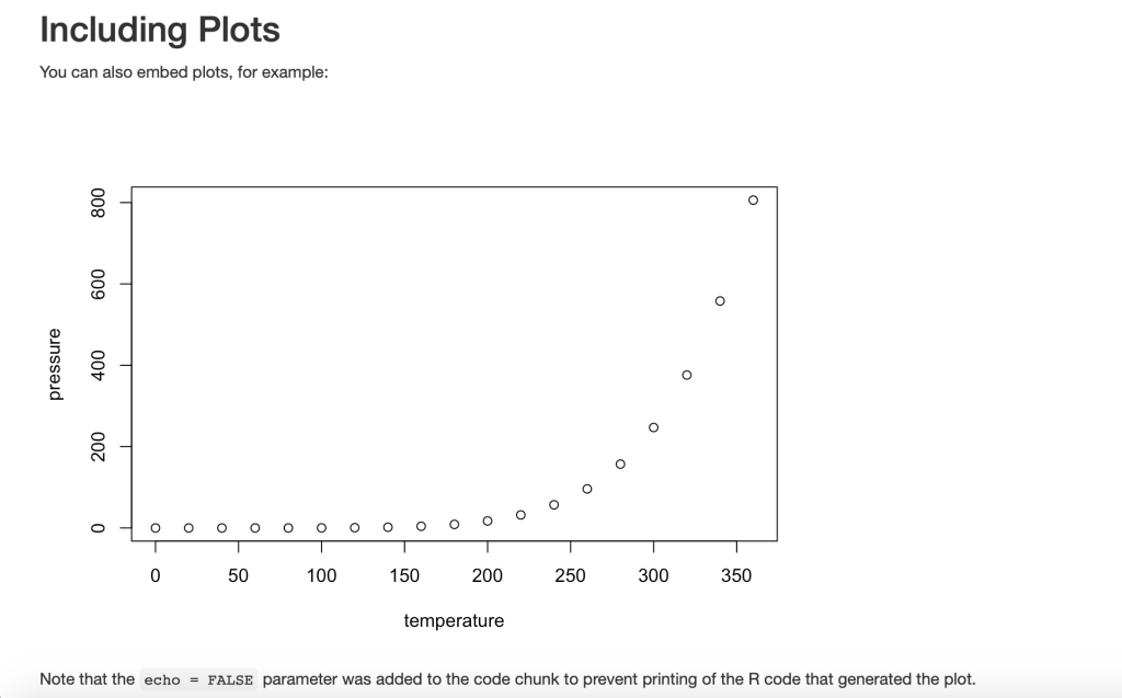
The basic R Studio Markdown example was formatted by HTML and knitted into this document:

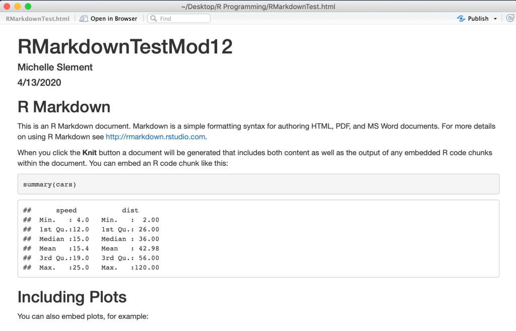
file://localhost/Users/michelleslement/Desktop/R%20Programming/RMarkdownTest.html

HTML Link

I think this is an amazing resource for coding in R and presenting your work.

In my other class I “compile” using this tool(little notebook looking icon) which I found to be similar to R Markdown:

GitHub Repository link:https://github.com/mslement/LawWordCloud

GitHub Repository link DESCRIPTION file: https://github.com/mslement/LawWordCloud/blob/master/DESCRIPTION

My desktop opening up a new R project and linking it to my desktop folder as a working directory and I tried to connect it to my GitHub:

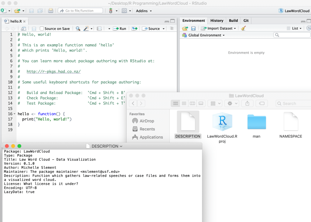
I am planning on updating the description file towards the end of my R package project once I have it fully running and complete.

Package: LawWordCloud
Type: Package
Title: Law Word Cloud – Data Visualization
Version: 0.1.0
Author: Michelle Slement
Maintainer: The package maintainer mslement@usf.edu
Description: Function which gathers law-related speeches or case files and forms them into a visualized word cloud.
License: What license is it under?
Encoding: UTF-8
LazyData: true

DESCRIPTION file

I found all the links to the articles about creating packages and projects in R to be very helpful this week. I also really enjoyed participating in the Zoom conference and seeing/hearing some of my online classmates.

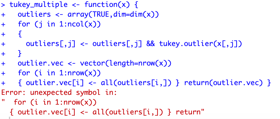
To begin, we were given the following code to debug:

I first ran the code to see if it compiled without any errors (spoiler… there were errors)

I removed the extra } and formatted the function to be more readable. This code ran without any errors and I was able to view the function with View(tukey_multiple).

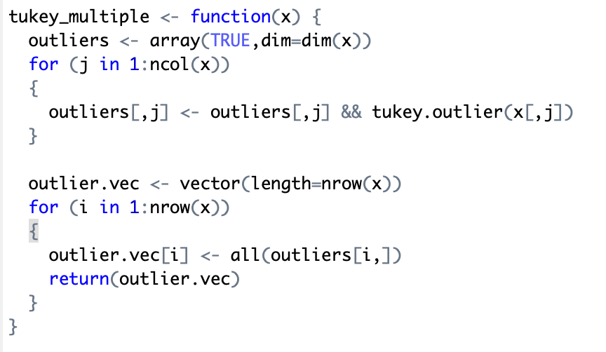
debug(tukey_multiple)

Code ran clear without any errors

This week was almost a review from last semester’s data visualization class which was nice! I chose the “Wool” dataset in carData package but I ended up downloading it through read.csv(“Wool.csv”) function after putting the .csv file in my R programming folder.

I originally chose this dataset because my sister lives in New Zealand on a sheep farm (not kidding) and my mom has been knitting wool clothes for my baby nephew.

https://vincentarelbundock.github.io/Rdatasets/datasets.html

Dataset website where I chose the “Wool” dataset

I noticed trends within the data and felt it was important to understand the column headings and variables I was working with so I looked them up. Below are the variables I will be working with for my three visualizations.

Data Visualization #1: Simple Histogram

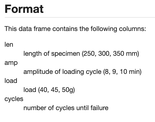
This simple histogram highlights how most wool, even if it has a higher length or thread count, will fail while washing cycles within the first 2000 cycles.

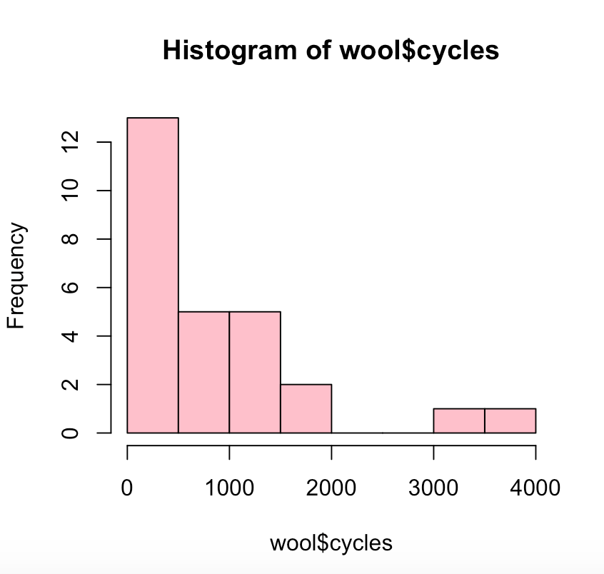
hist(wool$cycles, col=”pink”)

R Code

Data Visualization #2: Line/Point Graph

There was not a lot of linear data so I did not connect the data by a line. Instead I choice points to visualize the continuing theory that the higher length grants more cycles of washing pertaining to wool data.

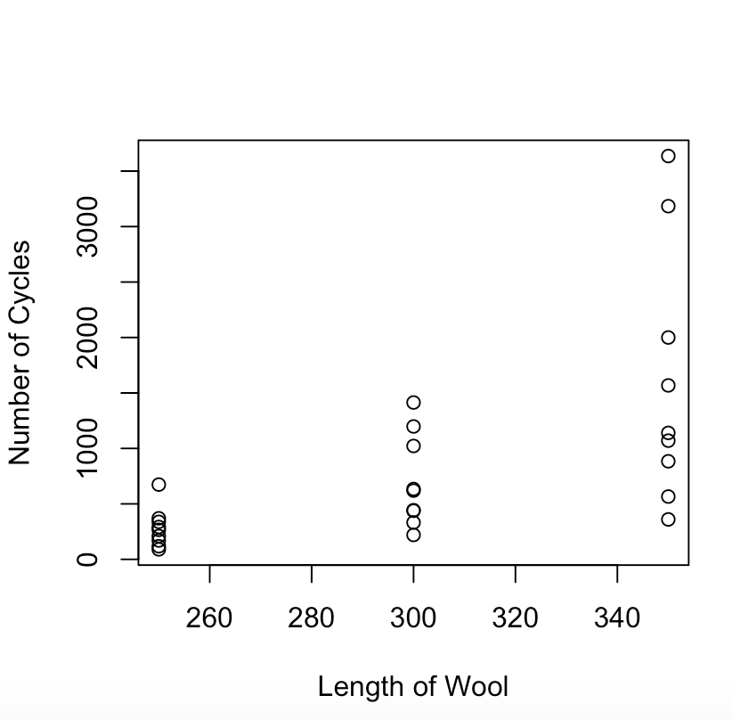
lineWool <- plot(wool$len, wool$cycles, type=”p”, xlab=”Length of Wool”, ylab=”Number of Cycles”)

R Code

I found this graph to be interesting as there is a pretty significantly varying distribution of cycles(~500 – ~4000) for the 350 length wool while the 250 length wool stayed at less than 1000 cycles.

Data Visualization #3: Faceting

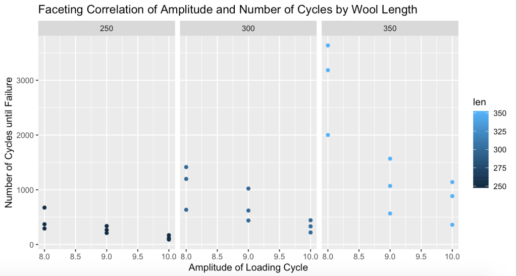
Faceting was my favorite type of visualization I learned last semester so I decided to include it in this module because I recognized that there were 3 distinct lengths of wool to facet and show their cycle failure patterns with.

> facet.wool <- ggplot(wool, aes(x=amp, y=cycles, col=len)) + xlab(“Amplitude of Loading Cycle”) +ylab(“Number of Cycles until Failure”) + ggtitle(“Faceting Correlation of Amplitude and Number of Cycles by Wool Length”) + geom_point()
> facet.wool + facet_grid(~wool$len)

R Code

GitHub Link: https://github.com/mslement/IntroRProgrammingSlement/blob/master/Module9Visualizations

This week’s assignment was pretty straightforward as we were given code to utilize and run through the steps given. Truthfully, I had to manipulate and change most of the given code on Canvas to be able to utilize it in my RStudio but everything ended up working out in the end.

Step 1 – Importing Data Set and StudentAverage

• 

Finishing the step we wrote a file for the output.

write.csv(StudentAverage,’StudentAverageSex.csv’)

R Code

Step 2 – “I” Student Data

Step 3 – Write the filtered data set and convert it to CSV file

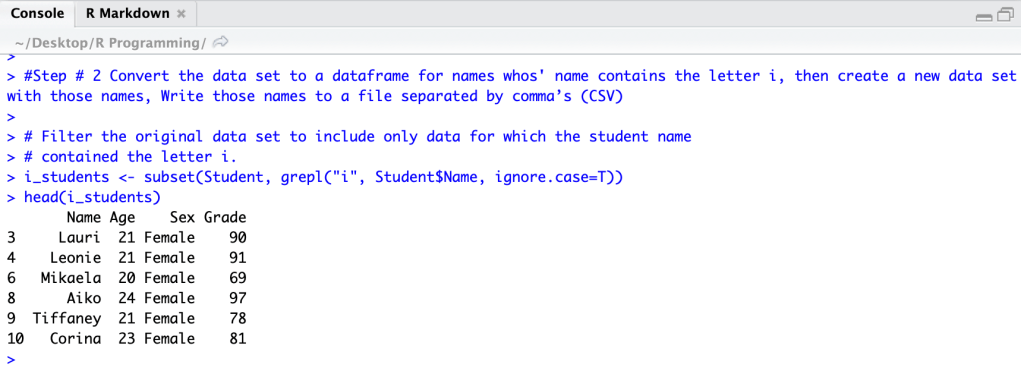
write.csv(i_students,’i_students.csv’)

R Code

Hint – Make sure to set your directory so you can find the saved files.

GitHub Link: https://github.com/mslement/IntroRProgrammingSlement/blob/master/Module8

Download any type of data (from the web or use datasets package) or create your own set.

data(“iris”)
head(iris)
Sepal.Length Sepal.Width Petal.Length Petal.Width Species
1 5.1 3.5 1.4 0.2 setosa
2 4.9 3.0 1.4 0.2 setosa
3 4.7 3.2 1.3 0.2 setosa
4 4.6 3.1 1.5 0.2 setosa
5 5.0 3.6 1.4 0.2 setosa
6 5.4 3.9 1.7 0.4 setosa
library(“pryr”, lib.loc=”/Library/Frameworks/R.framework/Versions/3.6/Resources/library”)

R Code

Then, on the second step, determine if generic function as discussed in this module can be assigned to your data set, and if not, why?

otype(iris)
[1] “S3”

R Code

S3 – Based on Example in Powerpoint

• 

S4 – Based on Example in Powerpoint

• 

Discussion Questions

How do you tell what OO system (S3 vs. S4) an object is associated with?

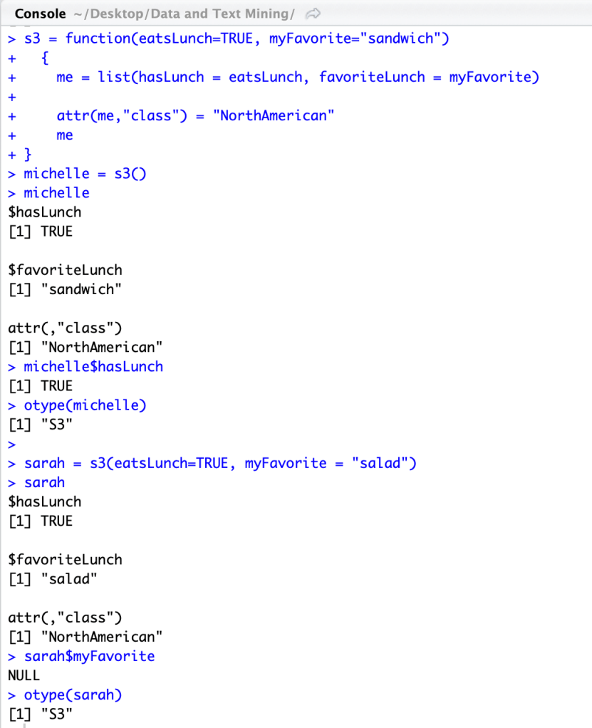
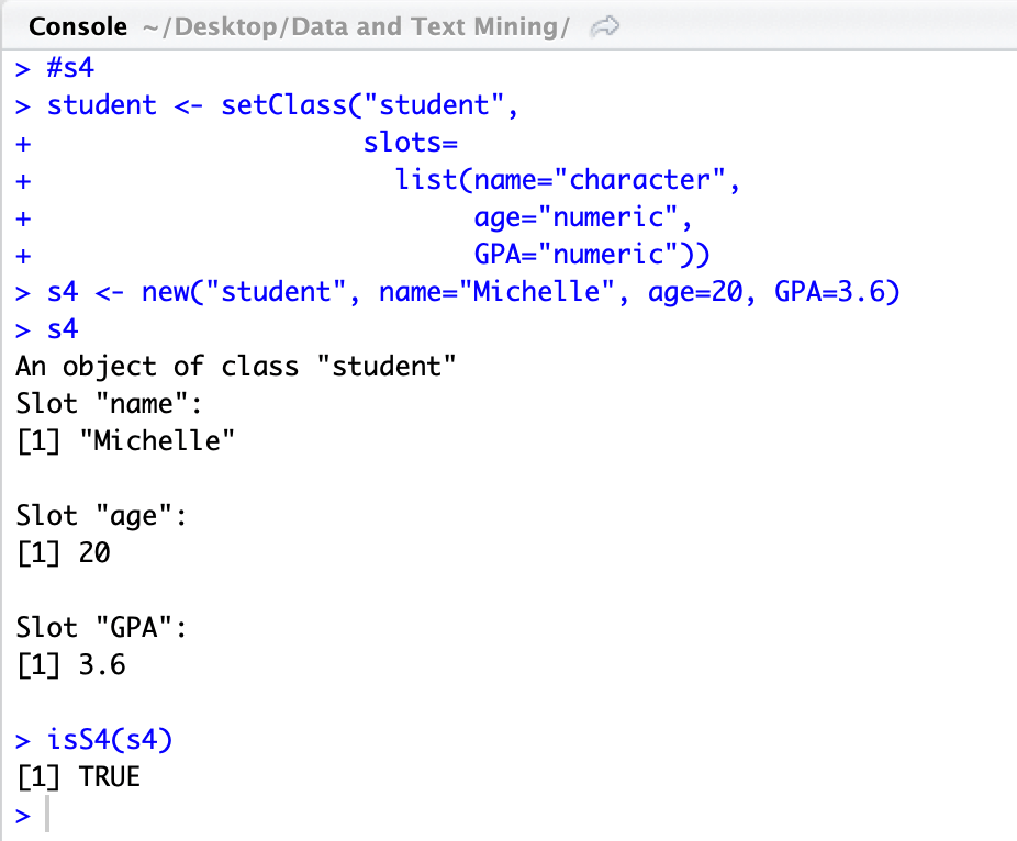
You can tell what OO system an object is associated with by how it was created and the methods used. You can also check with the functions otype(___) or isS4(___).

How do you determine the base type (like integer or list) of an object?

You can determine the base type of an object with the class() or typeof() functions.

What is a generic function?

The generic function f() is an operation function which dispatches methods and can be done by f.classname() in S3 and setMethod() in S4

What are the main differences between S3 and S4?

There are many differences between S3 and S4 besides using different functions for their operations such as f.classname() in S3 and then setMethod() in S4. Overall, S3 is single dispatch, more interactive and informal(simpler) while S4 is multi-dispatch, less interactive but more formal(structured) and rigorous.

My GitHub Repository- https://github.com/mslement/IntroRProgrammingSlement/blob/master/S3%20and%20S4

This week we continued to evaluate matrixes in R using two given matrix sets(A and B), a diagonal matrix (4, 1, 2, 3) and then create a copy of a given matrix.

1. Consider A=matrix(c(2,0,1,3), ncol=2) and B=matrix(c(5,2,4,-1), ncol=2).

A <- matrix(c(2,0,1,3), ncol=2)
A
[,1] [,2]
[1,] 2 1
[2,] 0 3
B <- matrix(c(5,2,4,-1), ncol=2)
B
[,1] [,2]
[1,] 5 4
[2,] 2 -1

R Code

a) Find A + B

add <- A + B
add
[,1] [,2]
[1,] 7 5
[2,] 2 2

R Code

b) Find A – B

substract <- A – B
substract
[,1] [,2]
[1,] -3 -3
[2,] -2 4

R Code

After playing around with different uses of diag(), I finally got #2:

2. Using the diag() function to build a matrix of size 4 with the following values in the diagonal 4,1,2,3.

m2 <-diag(x = c(4, 1, 2, 3), nrow=4, ncol=4, names = TRUE)
m2
[,1] [,2] [,3] [,4]
[1,] 4 0 0 0
[2,] 0 1 0 0
[3,] 0 0 2 0
[4,] 0 0 0 3

R Code

3. Generate the following matrix:

m3 <- diag(x = 3, nrow=5, ncol=5, names = TRUE)
m3[,1]<- 2
m3[1,]<- 1
diag(m3) <- 3
m3
[,1] [,2] [,3] [,4] [,5]
[1,] 3 1 1 1 1
[2,] 2 3 0 0 0
[3,] 2 0 3 0 0
[4,] 2 0 0 3 0
[5,] 2 0 0 0 3

R Code

Honestly, #3 was very difficult and I am not sure if I did it correctly but it matches the given matrix. But, I feel as though playing around with diag() function and matrix functions really helped me understand how they work. In my other class(data and text mining), I am given a data set and use the as.matrix() function but did not understand until this assignment what that function actually does.

I found this website super helpful: https://stat.ethz.ch/R-manual/R-devel/library/base/html/diag.html

This week we evaluated matrixes in R using two given matrix sets(A and B). Below is the R code console

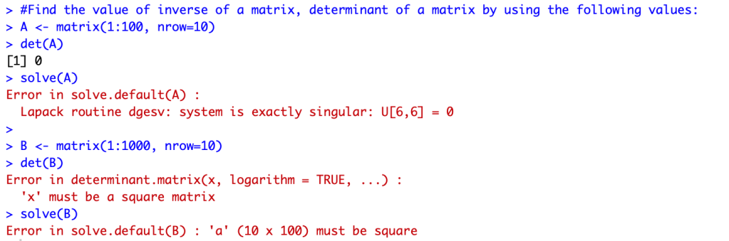
R provides with a lot of information as to why some codes did not work and resulted in an error. Most of the errors were a result of the dimensions of the two matrixes. To better understand I used the dim() function in R.

dim(A)
[1] 10 10
dim(B)
[1] 10 100

R Code

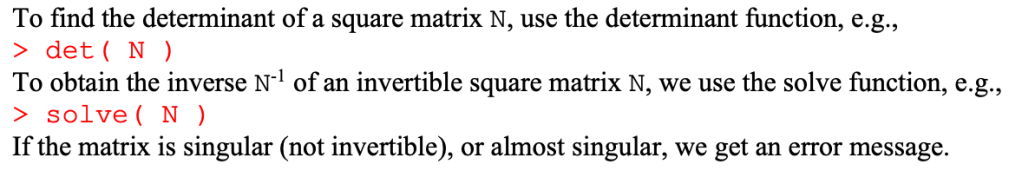
For Matrix A: the determinant worked because the matrix was a square (dimensions of 10×10); the inverse did not work and displayed an error because it was exactly singular

For Matrix B: due to the “nrow = 10” dimensions, the determinant was not able to be found as it is not a square (dimensions of 10×100); the aspect of the matrix not being a square also affected the inverse “solve” function

This week I evaluated this code in R and GitHub:

assignment2 <- c(16, 18, 14, 22, 27, 17, 19, 17, 17, 22, 20, 22)

myMean <- function(assignment2) { return(sum(assignment)/length(someData))}

myMean

The code complied and ran as follows:

>assignment2 <- c(16, 18, 14, 22, 27, 17, 19, 17, 17, 22, 20, 22)

>myMean <- function(assignment2) { return(sum(assignment2)/length(someData))}
>myMean
function(assignment2) { return(sum(assignment2)/length(someData))}

The code runs with no errors but the function calls sum(assignment) not sum(assignment2) so the mean would not be of the data in the assignment2 vector. The function does not return the value of myMean, but rather returns a copy of the function. “someData” needs to be defined as a value (such as 12) or the length of assignment2 vector.

GitHub link: https://github.com/mslement/IntroRProgrammingSlement/blob/master/myMean